Cloud evolution

Evolution equations

The evolution of the cloud (boson mass \(m_b = \hbar /(\mu c^2)\)) is described within the quasiadiabatic approximation by a system of coupled differential equations (see e.g. arXiv:1411.0686). These determine the rate of change of the cloud’s mass (\(\dot{M}_c= \dot{E}_c/c^2\)) and angular momentum (\(\dot{J}_c\)) in terms of the power (\(P_{gw}\)) and angular momentum (\(\dot{J}_{gw} = P_{gw}/\omega_R\)) radiated in GWs and the black-hole parameters (\(M, J\)), which is possibly affected by accretion (\(\dot{M}_{\rm Acc}, \dot{J}_{\rm Acc}\)).

\begin{align} \dot{M}_c^{\rm (sr)} &= 2 M_c \omega_I\\ \dot{M} &= - \dot{M}_c^{\rm (sr)} + \dot{M}_{\rm Acc}\\ \dot{M} + \dot{M}_c &= - P_{gw}/c^2 + \dot{M}_{\rm Acc} \\ \dot{J} &= - m c^2 \dot{M}_c^{\rm (sr)} / \omega_R + \dot{J}_{\rm Acc}\\ \dot{J} + \dot{J}_c &= - m P_{gw}/\omega_R + \dot{J}_{\rm Acc}\, , \end{align}

where \(\dot{M}_c^{\rm (sr)}\) is the change in the cloud mass due to superradiance only (\(\dot{M}_c = \dot{M}_c^{\rm (sr)} - P_{gw}/c^2\)), and \(\omega = \omega_R + i \omega_I\) is the boson field frequency. In the case of no accretion, this simplifies to

\begin{align} \dot{M} &= - 2 M_c \omega_I\\ \dot{M} + \dot{M}_c &= - P_{gw}/c^2 \\ \dot{J} &=- 2 m c^2 M_c \omega_I / \omega_R \\ \dot{J} + \dot{J}_c &= - m P_{gw}/\omega_R \, . \end{align}

we can solve these equations numerically, starting from some initial parameters \((M_0, J_0, M_{c,0}, J_{c,0})\).

Numerical setup

Set up the above system of DE’s in a way ammenable to numerical treatment.

No accretion

Define dimensionless \((x, y, j^x, j^y, {\cal P}, w, \tau)\) quantities such that

\begin{align} M &= \alpha x\\ M_c &= \alpha y \\ J &= \beta j^x\\ J_c &= \beta j^y\\ P_{gw} &= \gamma {\cal P}\\ \omega &= w \mu\\ t &= \epsilon \tau\, . \end{align}

We will make sure these are dimensionless by defining the dimensionful factors

\begin{align} \alpha &= M_0 \\ \beta &= M_0 c^2 \mu^{-1} \\ \gamma &= M_0 c^2 \mu \\ \epsilon &= \mu^{-1}\, , \end{align}

and letting \(\mu = \hbar/(m_b c^2)\) be the Compton frequency associated with the boson rest mass, \(m_b\). We will also let \(M_0\) be the initial black-hole mass. Note that then we have:

\begin{align} a &= \frac{c j_x \epsilon}{x} \\ \chi &= \frac{j_x}{x^2} \frac{\epsilon}{T_0}\, , \end{align}

where we have defined the horizon crossing time \(T_0 = G M_0/c^3\). Also note that the SR condition is saturated when

\begin{equation} \left( \frac{2}{m} \frac{T_0}{\epsilon}\right)^2 = \frac{j_x}{x^2\left(mx-j_x\right)} \end{equation}

With the above notation, the BHB evolution equations become:

\begin{align} x' &= -2 w_I y\\ x' + y' &= -{\cal P}\\ (j^x)' &= -2 m w_I w_R^{-1} y\\ (j^x)' + (j^y)' &= -m w_R^{-1} {\cal P} \end{align}

for \(m\) the boson magnetic quantum number (\(m=1\) for dominant scalar level), and where the prime denotes \({\rm d}/{\rm d}\tau\). We may turn these into finite-difference equations to obtain:

\begin{align} x_{i+1} &= x_i -2 w^I_i y_i \delta \tau \\ y_{i+1} &= y_i + 2 w^I_i y_i \delta\tau -{\cal P}_i \delta \tau\\ j^x_{i+1} &= j^x_i -2 m (w^I_i/ w^R_i) y_i \delta \tau\\ j^y_{i+1} &= j^y_i + m \left( 2 w^I_i y_i - {\cal P}_i\right)\delta \tau / w^R_i \end{align}

These can be evolved from \((x_0, y_0, j^x_0, j^y_0)\) until the SR spin threshold is reached. The final state can then be converted into physical units using the scalings defined above.

Adding back accretion

In the presence of accretion, we may define the dimensioless accretion mass and angular momentum rates:

\begin{align} {\cal M}_a ' &\equiv c^2 \gamma^{-1} \dot{M}_{\rm Acc} = (M_0 \mu)^{-1} \, \dot{M}_{\rm Acc} \\ {\cal J}_a ' &\equiv\, \epsilon \beta^{-1} \dot{J}_{\rm Acc} = (M_0 c^2)^{-1} \dot{J}_{\rm Acc} \, , \end{align}

so that the evolution equations become:

\begin{align} x' &= -2 w_I y + {\cal M}_a '\\ x' + y' &= -{\cal P} + {\cal M}_a '\\ (j^x)' &= -2 m w_I w_R^{-1} y + {\cal J}_a' \\ (j^x)' + (j^y)' &= -m w_R^{-1} {\cal P} + {\cal J}_a' \, . \end{align}

The corresponding finite-difference equations are:

\begin{align} x_{i+1} &= x_i -2 w^I_i y_i \delta \tau + {\cal M}_a' \delta\tau \\ y_{i+1} &= y_i + 2 w^I_i y_i \delta\tau -{\cal P}_i \delta \tau \\ j^x_{i+1} &= j^x_i -2 m (w^I_i/ w^R_i) y_i \delta \tau + {\cal J}_a' \delta\tau\\ j^y_{i+1} &= j^y_i + m \left( 2 w^I_i y_i - {\cal P}_i\right)\delta \tau / w^R_i \, , \end{align}

assuming that the accretion rate is constant. Note that accretion only affects the BH quantities (\(x, j^x\)) by construction, because we assumed no direct interaction between the cloud and the accretion disk.

Evolving forward

%pylab inline
import gwaxion

Populating the interactive namespace from numpy and matplotlib

Final state

The gwaxion package can use the above equations (ignoring cloud angular momentum and GW power) to automatically obtain the final (post-superradiance) properities of a given black-hole–boson (BHB) system. Simply make sure this feature is turned on through the evolve argument when creating a BosonCloud object.

Here’s an example for the \(\ell=m=1\) cloud from pre-superradiance BH with \(60\, M_\odot\) and \(\chi=0.7\), and a boson such that \(\alpha=0.176\).

c = gwaxion.BosonCloud.from_parameters(1, 1, 0, evolve=True, m_bh=60,
                                       chi_bh=0.7, alpha=0.176)

Print some post-superradiance parameters, which will be internally computed using the above DEs.

l = [
    "Final BH mass: %.2f Msun" % c.bhb_final.bh.mass_msun,
    "Final BH spin: %.3f" % c.bhb_final.bh.chi,
    "Final BH J: %.2e" % c.bhb_final.bh.angular_momentum,
    "Final alpha: %.3f" % c.bhb_final.alpha,
    "Final cloud mass: %.2f Msun" % c.mass_msun
]
print('\n'.join(l))

Final BH mass: 58.89 Msun
Final BH spin: 0.617
Final BH J: 1.89e+45
Final alpha: 0.173
Final cloud mass: 1.11 Msun

If the DE evolution is turned off with evolve=False, then the code approximates the final BH parameters using Eqs. (25) and (26) in arXiv:1706.06311, with constant \(\alpha\) corresponding to the initial BH parameters.

The result is slightly different:

c_approx = gwaxion.BosonCloud.from_parameters(1, 1, 0, evolve=False, m_bh=60,
                                              chi_bh=0.7, alpha=0.176)

l = [
    "Final BH mass: %.2f Msun" % c_approx.bhb_final.bh.mass_msun,
    "Final BH spin: %.3f" % c_approx.bhb_final.bh.chi,
    "Final BH J: %.2e" % c_approx.bhb_final.bh.angular_momentum,
    "Final alpha: %.3f" % c_approx.bhb_final.alpha,
    "Final cloud mass: %.2f Msun" % c_approx.mass_msun
]
print('\n'.join(l))

Final BH mass: 59.21 Msun
Final BH spin: 0.624
Final BH J: 1.93e+45
Final alpha: 0.174
Final cloud mass: 0.79 Msun

Evolution

We can study the evolution of the system during the superrandiance process by looking at the properties of the BHB system over time. To do this with gwaxion we need to call the DE solver directly.

We can start from the BosonCloud object we defined above, and call the internal method _evolve_instability()

bhb_final, (xs, jxs, ys, inv_wRs, wIs, sr_conds, times)  = c._evolve_instability()

The bhb_final object contains the final state of the evolution, and should give the same results as above, e.g.

l = [
    "Final BH mass: %.2f Msun" % bhb_final.bh.mass_msun,
    "Final BH spin: %.3f" % bhb_final.bh.chi,
    "Final BH J: %.2e" % bhb_final.bh.angular_momentum,
    "Final alpha: %.3f" % bhb_final.alpha,
]
print('\n'.join(l))

Final BH mass: 58.89 Msun
Final BH spin: 0.617
Final BH J: 1.89e+45
Final alpha: 0.173

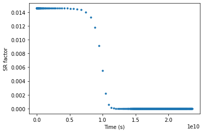
The other outputs contain the quantities computed at each step of the DE evolution: \(x\), \(j^x\), \(y\), \(w_R^{-1}\), \(w_I\), defined above; as well as the “SR factor”, which vanishes when SR stops; and time.

For example, as time goes by, the superradiance quickly saturates until it stops:

scatter(times, sr_conds, marker='.')
ylabel('SR factor');
xlabel('Time (s)');

As this happens, the cloud grows in mass at the expense of the BH:

plot(times, ys/xs)
axvline(6E9, ls='--', c='k')
axvline(6E9+1500*c.number_growth_time, ls='--', c='k')
xlabel('Time (s)');
ylabel(r'$M_c/M_{\rm BH}$');

Note that the timesteps are not equally separated, since the solver adapts the interval according to the evolution of the system:

plot(times)
xlabel('Steps');
ylabel('Time (s)');